Time-reversal refocusing in random media

For my MVA inverse-problems project, I simulated a wave emitted near a source, recorded at a distant mirror, and sent back through the same medium. The question was how accurately the returning wave could concentrate around its starting point. I first studied the effect of the mirror aperture in a homogeneous medium, then introduced random fluctuations and compared the resulting focal profiles.

The simulations in motion

These animations reconstruct a time-dependent pulse by combining 100 frequencies. The left panel shows the outward propagation, then plays that recording backwards; the right panel shows the computed return through the medium. Colors represent signed wave amplitude.

Homogeneous medium, with Gaussian mirror scale \(r_M=20\).

One random medium realization, with fluctuation strength \(\sigma=1\) and Gaussian mirror scale \(r_M=5\).

The two animations use different mirror apertures. The comparisons at fixed aperture are shown in the plots below.

A model for propagation

The simulation has one longitudinal coordinate \(z\) and one transverse coordinate \(x\). For a fixed angular frequency \(\omega\), I write the wave as a slowly varying envelope \(\phi(z,x)\) multiplying a plane wave \(e^{ikz}\), where \(k=\omega/c_0\). Neglecting the second longitudinal derivative of the envelope gives the paraxial equation

\[\partial_z\phi =\frac{i}{2k}\partial_x^2\phi +\frac{ik}{2}\mu(z,x)\phi, \qquad \phi(0,x)=e^{-x^2/r_0^2}.\]

The first term describes diffraction; the second describes the fluctuations of the medium. Setting \(\mu=0\) gives the homogeneous reference problem. This is a directional propagation model: the numerical results concern this approximation rather than a full wave-equation simulation.

I implemented a split-step Fourier solver. Over a distance \(h\), it applies diffraction in Fourier space, then refraction in physical space:

\[\phi(z+h,x)\approx e^{ikh\mu(z,x)/2}\, \mathcal F^{-1}\!\left[ e^{-ih\kappa^2/(2k)}\mathcal F[\phi(z,\cdot)](\kappa) \right](x).\]

Here \(\kappa\) is the transverse spatial frequency. Each substep is a simple phase multiplication. Their composition approximates the coupled evolution because diffraction and refraction do not generally commute. The homogeneous Gaussian solution also has an analytical expression, which I used to compare the numerical transmitted and refocused profiles against a known solution.

Recording and sending the wave back

At \(z=L\), the mirror weights the recorded field with a Gaussian window of scale \(r_M\). For a monochromatic wave, time reversal is implemented through complex conjugation:

\[\phi_{\mathrm{tr}}(L,x) =M(x)\overline{\phi(L,x)}, \qquad M(x)=e^{-x^2/r_M^2}.\]

The return calculation traverses the same medium layers in reverse order. It also reverses the order of the two numerical substeps. The plots use an unfolded distance: \(0\leq z\leq L\) represents the outward journey, and \(L\leq z\leq2L\) the return. Thus \(z=2L\) corresponds physically to arriving back at the source plane.

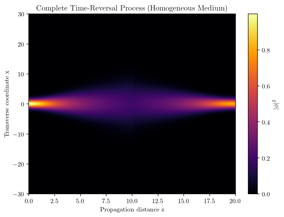
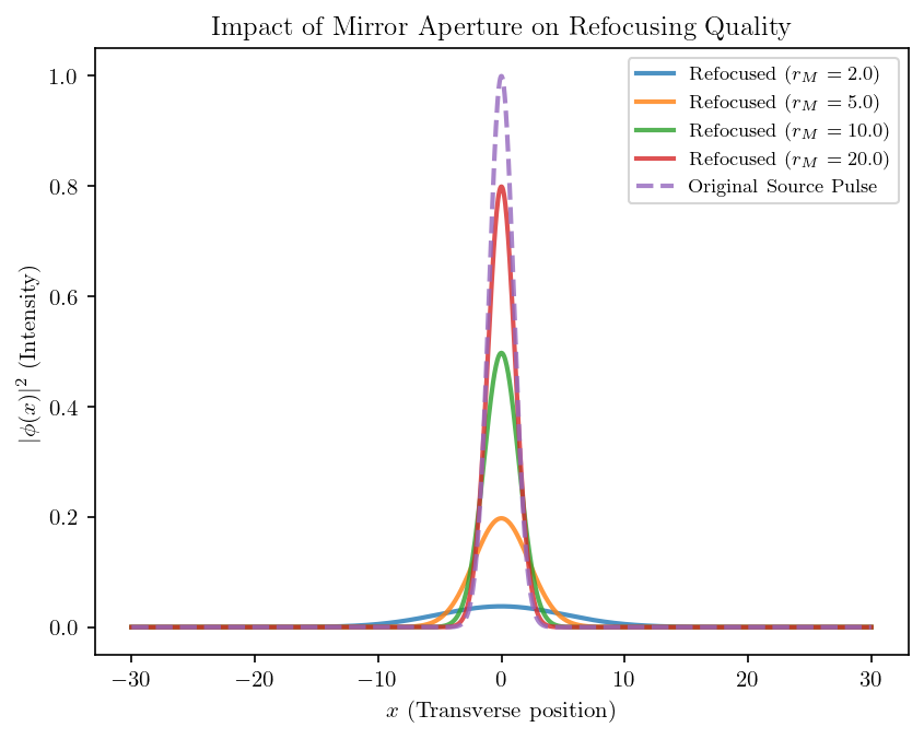
Intensity during the outward and return propagation in a homogeneous medium — Complete homogeneous experiment with \(L=10\) and \(r_M=20\). The beam spreads before the mirror at unfolded distance \(z=10\), then concentrates again near \(x=0\).

The mirror changes what can be returned. A small \(r_M\) strongly attenuates the field away from its center; increasing \(r_M\) preserves more of the recorded profile. In the homogeneous experiment below, this produces a narrower, higher refocused peak, closer to the original Gaussian source.

Homogeneous refocusing for four Gaussian mirror sizes, compared with the initial source — Numerical intensities at the source plane for \(r_M=2,5,10,20\). The dashed curve is the initial source intensity. A Gaussian mirror has a smooth window, so \(r_M\) is an aperture scale rather than a hard boundary.

What changes in a random medium

I modeled the medium as independent layers of thickness \(z_c\). Within each layer, \(\mu_n(x)\) is a zero-mean Gaussian process with covariance

\[\mathbb E[\mu_n(x)\mu_n(x')] =\sigma^2\exp\!\left(-\frac{(x-x')^2}{x_c^2}\right).\]

The parameters separate the strength of the fluctuations, \(\sigma\), from their transverse scale, \(x_c\). The comparison below varies \(\sigma\) and the mirror size while keeping \(z_c=1\) and \(x_c=4\).

To interpret it, the order of averaging matters. The notebook averages the complex refocused fields over 100 realizations, then plots the squared magnitude:

\[\overline\phi_N(x)=\frac1N\sum_{j=1}^{N}\phi_{\mathrm{tr}}^{(j)}(2L,x), \qquad I_{\mathrm{coh},N}(x)=|\overline\phi_N(x)|^2.\]

This measures the part of the field that survives averaging across media. It differs from averaging the individual intensities, \(N^{-1}\sum_j\lvert\phi_{\mathrm{tr}}^{(j)}\rvert^2\).

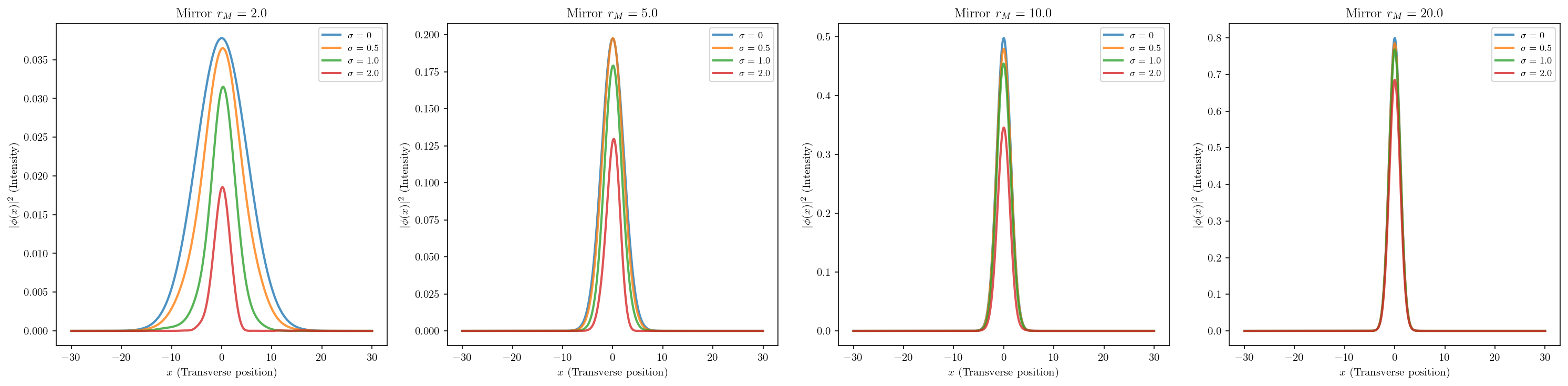
Squared magnitude of the averaged refocused field for four mirror sizes and four fluctuation strengths — Refocused sample-mean profiles. Each panel fixes \(r_M\) and compares \(\sigma=0,0.5,1,2\). The panels use different vertical scales. Open the figure to see the individual panels at full size.

For the smallest mirror, increasing the fluctuations visibly narrows the central peak, while also lowering its height. The width changes much less for the largest mirror. Here, “super-resolution” refers to that narrower mean profile relative to the homogeneous experiment with the same mirror. These curves do not establish that every individual realization has a sharper focus, or that a narrower peak returns more energy.

Source code and numerical experiments.